Outlier Detection

Outlier detection can be achieved through some very simple, but powerful algorithms. All the examples here are either density or distance measurements. The code here is non-optimized as more often than not, optimized code is hard to read code. Additionally, these measurements make heavy use of K-Nearest-Neighbors. Consequently, they not be as useful at higher dimensions.

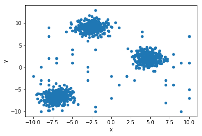
First, lets generate some data with some random outliers.

%matplotlib inline
# Generate some fake data clusters
from sklearn.datasets import make_blobs
from matplotlib import pyplot
from pandas import DataFrame
import random
import numpy as np

r_seed = 42

# Generate three 2D clusters totalling 1000 points 
X, y = make_blobs(n_samples=1000, centers=3, n_features=2, random_state=r_seed)
random.seed(r_seed)
random_pts = []

# Generate random noise points that could be or could not be close to the clustered neighborhoods
for i in range(50):
    random_pts.append([random.randint(-10, 10), random.randint(-10, 10)])

X = np.append(X, random_pts, axis=0)

df = DataFrame(dict(x=X[:,0], y=X[:,1]))
df.plot(kind='scatter', x='x', y='y')
pyplot.show()

The Algorithms

Four separate algorithms are shown below:

• Local Outlier factor (LoF): This is a density metric that determines how dense a points local neighborhood is. The neighborhood is determined via the K nearest neighbors
• Local Distance-based outlier factor (LDoF): This is a density + distance algorithm that is similar to LoF, but instead of worrying about neighborhood density, it looks at how far a point is from the perceived center of the neighborhood.
• K^th Nearest Neighbors Distance (K^thNN): A distance metric that looks at how far away a point is from its Kth nearest neighbor
• K Nearest Neighbors Total Distance (TNN): A distance metric that is the averaged distance to the K nearest neighbors

Kth Nearest Neighbor Distance (K^thNN)

This is a very intuitive measure. How far away are you from your K^th neighbor? The farther away, the more likely you are to be an outlier from the set.

from sklearn.neighbors import NearestNeighbors

k = 10

knn = NearestNeighbors(n_neighbors=k)

knn.fit(X)
# Gather the kth nearest neighbor distance
neighbors_and_distances = knn.kneighbors(X)
knn_distances = neighbors_and_distances[0]
neighbors = neighbors_and_distances[1]
kth_distance = [x[-1] for x in sk_knn_distances]

Average distance to K Nearest Neighbors (TNN)

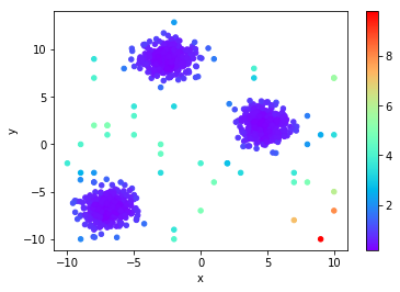
Very similar to K^thNN, but we average out all the distances to the K nearest neighbors. Since K^thNN only takes a single neighbor into consideration, it may miss certain outliers that TNN finds.

# Gather the average distance to each points nearest neighbor 
tnn_distance = np.mean(knn_distances, axis=1)

Notice the point in the upper-right corner, TNN determines that it is more likely an outlier due to how far it is from all its neighbors.

Local Distance-based Outlier Factor (LDoF)

This algorithm is slightly more complicated, though not by much.

The paper explaining it in depth is here.

Here is the simplified version.

We have already calculated one part of this algorithm through TNN. Lets call keep this value as TNN(x), for some point x.

The other part is what the paper calls the “KNN inner distance”. This is the average of all the distances between all the points in the set of K nearest neighbors, referred to here as KNN(x).

So, the Ldof(x) = TNN(x)/KNN_Inner_distance(KNN(x))

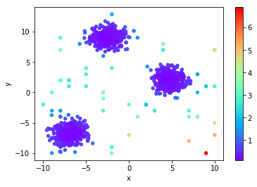
This combination makes this method a density and a distance measurement. The idea is that a point with a LDoF score » 1.0 is well outside the cloud of K nearest neighbors. Any point with an LDoF score less than or “near” 1.0 could be considered “surrounded” via the cloud of neighbors.

# Gather the inner distance for pts
def knn_inner_distance(pts):
    summation = 0
    for i in range(len(pts)):
        pt = pts[i]
        for other_pt in pts[i:]:
            summation = summation + np.linalg.norm(pt - other_pt)
    return summation / (k * (k - 1))

inner_distances = [knn_inner_distance(X[ns]) for ns in neighbors]

ldofs = [x/y for x,y in zip(tnn_distance, inner_distances)]

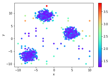
You can notice the effect of the “cloud” idea. All the points between the clusters are marked with a much lower probability of being an outlier, while those outside the cloud have a much higher likelihood.

Local Outlier Factor (LoF)

LoF is a density focused measurement. The core concept of this algorithm is reachability_distance. This is defined as reachability_distance(A, B) = max{distance(A,B), KthNN(B)}. In other words, it is the true distance between A and B, but it has to be AT LEAST the distance between B and its K^th nearest neighbor.

This makes reachability_distance asymmetrical. Since A and B have a different set of K nearest neighbors, their own distances to their K^th neighbor will differ.

Using reachability_distance we can calculate the local_reach_density to point’s neighborhood density.

For some point x, its local_reach_density is 1 divided by the average of all the reachability_distance(x, y) for all y in KNN(x), i.e. the set of x’s K nearest neighbors.

Armed with this, we can then compare point x’s local_reach_density to that of its neighbors to get the LoF(x).

The wikipedia article on lof gives an excellent, succinct mathematical and visual explanation.

local_reach_density = []
for i in range(X.shape[0]):
    pt = X[i]
    sum_reachability = 0
    neighbor_distances = knn_distances[i]
    pt_neighbors = neighbors[i]
    for neighbor_distance, neighbor_index in zip(neighbor_distances, pt_neighbors):
        neighbors_kth_distance = kth_distance[neighbor_index]
        sum_reachability = sum_reachability + max([neighbor_distance, neighbors_kth_distance])
        
    avg_reachability = sum_reachability / k
    local_reach_density.append(1/avg_reachability)

local_reach_density = np.array(local_reach_density)
lofs = []
for i in range(X.shape[0]):
    pt = X[i]
    avg_lrd = np.mean(local_reach_density[neighbors[i]])
    lofs.append(avg_lrd/local_reach_density[i])

# Or just use
# from sklearn.neighbors import LocalOutlierFactor